Mixed-Effects Models
One of the main assumptions of regression is independence of observations. What this means is we don’t want to measure the same observation twice, or deal with connected observations. We see this a lot in longitudinal studies or studies where groups are present. If we violate this assumption, our coefficients and p-values aren’t going to reliable; they could be inflated giving us false information on what is significant. How can we deal with this issue??? One way that we’ll go over today is the mixed-effects model!
Mixed-Effects Model Run-Down
The regression models we’ve developed previously all indicate effects of each predictor on the dependent variable. We can see the effect through the coefficient estimate. This effect is fixed for all observations. If the coefficient estimate is 3, that indicates that for every one unit increase in x, our predictor increases by 3. The model uses the same fixed effect for every observation.
Now let’s think of a longitudinal study. Let’s say, we’ll predict height over time of NBA players, from age 2 to age 18. We can try to get one fixed estimate of how age effects height, but that’s not a great way to measure this… Players have different baseline heights (you could be an unusually tall 2 year old compared to the rest of the sample) or have different rates of increase in height. We can account for this with random effects.
A mixed-effects model gets its name because it has fixed effects that impact the whole sample as well as random effects that account for the variation in each group (the groups in that case, would be the players). We can combine these fixed and random effects to get a sort-of unique regression line for each group.
We can also build upon mixed-effects models, adding in different underlying correlation and variance structures to better account for what we see in our residuals, allowing us to relax our assumptions of homogenous variance. All of this makes mixed-effects models great for working with repeated-measure and group studies.
Example and Data
The example I thought up for this lesson would be a longitudinal project where we take a look at the first four seasons of all Pacer rookies going back to the 1999-2000 season. We’ll build a mixed-effects model to predict win shares using the variables season number (a measure of time), what round the player was drafted, and the age the player was during their rookie season. We’ll be able to use this model for both inference as well as making predictions on the Pacer players who just finished up their rookie year.
The data we’ll scrape is from basketball reference. We’ll be scraping from multiple tables, so bear with me. As per usual with basketball reference, there are some intracacies with getting the info; I won’t make note of every edit, but I do make notes on prevalant pieces of scraping information. The first info we’ll grab is any player on the Pacer page who was listed as a rookie within our time-frame.
library(rvest)
library(dplyr)

pacer.rookies<-
  #using lapply to loop through the years 2000-2018
  lapply(2000:2018, function(x)
    #we'll be pasting the years into the Pacer team page url
    paste("https://www.basketball-reference.com/teams/IND/",x,".html",
          sep = "") %>%
      read_html(xpath='//*[@id="roster"]') %>%
      html_table() %>%
      .[[1]] %>%
      `colnames<-` (make.names(colnames(.))) %>%
      #we'll filter on the experience column for anyone labeled as "R"
      # for rookie
      filter(Exp=="R") %>%
      mutate(Rookie.Season=x)
    ) %>%
  bind_rows() %>%
  mutate(Player=gsub("\\s*\\([^\\)]+\\)", "", Player)) %>%
  select(Player, Rookie.Season)
Next, we’ll grab all of the stats for these players.
pacer.stats<-
  lapply(2000:2018, function(x)
  #loop through the advanced stat page to get win shares from 2000-2018
  paste("https://www.basketball-reference.com/leagues/NBA_",x,
        "_advanced.html",
        sep = "") %>%
  read_html() %>%
  html_node(xpath='//*[@id="advanced_stats"]') %>%
  html_table() %>%
  `colnames<-` (make.names(colnames(.), unique = T)) %>%
  mutate(Season=x) %>%
  distinct(Player, .keep_all = T)
) %>%
  bind_rows() %>%
  #filter on anyone that was a rookie with the pacers
  filter(Player %in% pacer.rookies$Player) %>%
  merge(pacer.rookies, by="Player") %>%
  #finding season number; adding 1 so it doesn't start at 0
  mutate(Season.Number=(Season-Rookie.Season)+1)
Finally, we’ll get draft information. I take this info and make reference dataframes for players drafted in the first and second round. I also went back a couple of additional years, just in case someone was drafted earlier, but didn’t start playing until 1999-2000.
draft<-
  lapply(1995:2017, function(x)
    #loop throught the draft page from 1995-2017
    paste("https://www.basketball-reference.com/draft/NBA_", x, ".html",
          sep="") %>%
  read_html() %>%
  html_node(xpath='//*[@id="stats"]') %>%
  html_table() %>%
  `colnames<-` (.[1,]) %>%
  `colnames<-` (make.names(colnames(.), unique = T)) %>%
  .[-1,] %>%
  #round 2 is listed as a row; every row after it is a 2nd rounder
  mutate(Round=ifelse(as.numeric(rownames(.))>
                      as.numeric(rownames(.[.$Player=="Round 2",])),
                      "Round 2", "Round 1")) %>%
  filter(Player != "Player") %>%
  filter(Player != "Round 2") %>%
  select(Player, Round)
  ) %>%
  bind_rows()

#create reference dataframes for 1st rounders and second rounders
round1<-
  draft %>%
  filter(Round=="Round 1")
round2<-
  draft %>%
  filter(Round=="Round 2")
Now that we scraped all of that information, we can put it all together into one dataframe!
pacer.stats<-
  pacer.stats %>%
  #have to rename joe young because he has a different name in the draft
  # dataframe
  mutate(Player=ifelse(Player=="Joe Young", "Joseph Young", Player)) %>%
  #new column for when the player was drafted
  mutate(Round=ifelse(Player %in% round1$Player, "Round 1",
                      ifelse(Player %in% round2$Player, "Round 2",
                             "Undrafted"))) %>%
  #filter for only the first four seasons
  filter(Season.Number<=4) %>%
  #merging with made up dataframe to get age player was as a rookie
  merge(pacer.stats %>%
          filter(Season.Number==1) %>%
          select(Player, Age) %>%
          rename(Rookie.Age=Age), by="Player") %>%
  mutate(WS=as.numeric(WS),
         Rookie.Age=as.numeric(Rookie.Age))
Looking at Our Data
Let’s take a look at our data to try and make some initial insights. Let’s first look at how win shares change over time by players in each round. The regression lines for round 1 and 2 have a similar slope, but round 1 has higher average predictions over time. Interestingly, the regression line for undrafted players has a negative slope as time increases.
library(ggplot2)

pacer.stats %>%
  ggplot(aes(x=Season.Number, y=WS, col=Round)) +
  stat_smooth(method="lm", se=F) +
  geom_jitter(alpha=.5, width = .2)
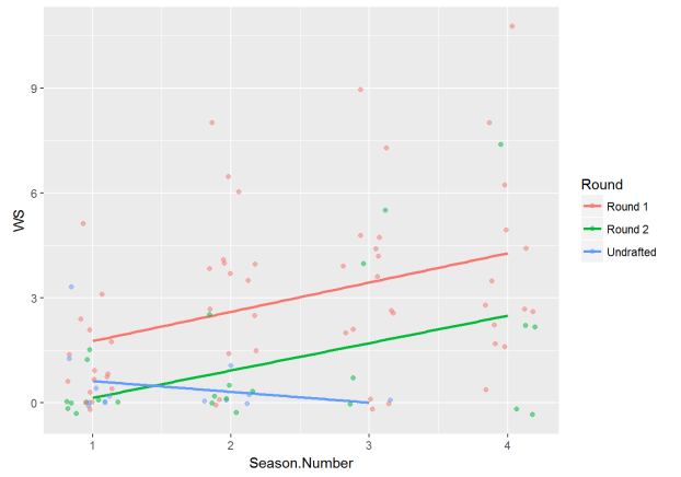
We can get a better idea of the effect of round via a boxplot. The median win shares value is much higher for round 1 players while round 2 and undrafted players are pretty low and similar.
pacer.stats %>%
  ggplot(aes(x=Round, y=WS)) +
  geom_jitter(width = .2) +
  geom_boxplot(alpha=.3)
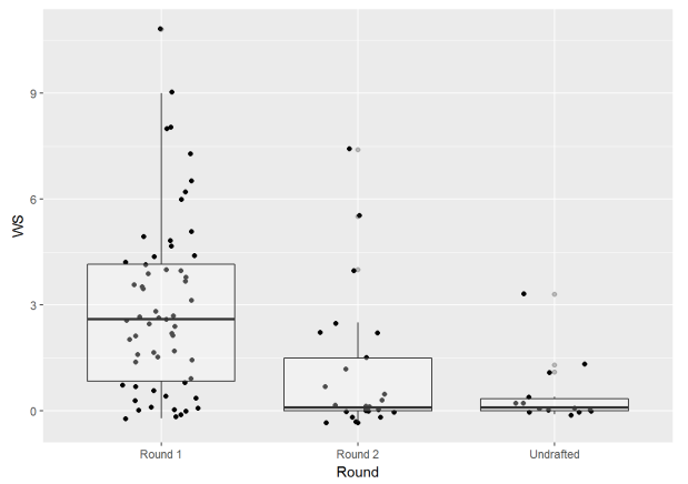
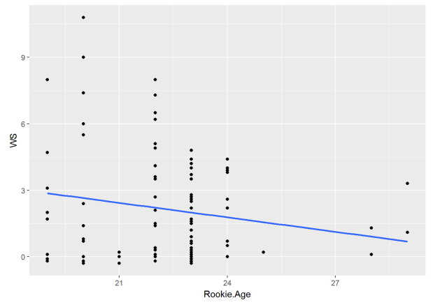
If we look at rookie age and win shares, we see a negative relationship. Players who were drafted older, tend not to produce as many win shares.
pacer.stats %>%
  ggplot(aes(x=Rookie.Age, y=WS)) +
  geom_point() +
  geom_smooth(method = "lm", se=F)
Developing a Mixed-Effects Model
With an idea of the relationships of our data, let’s build a mixed-effects model to predict win shares using season number, round drafted and rookie age. We’ll start off fairly simple with the random effects, only including a random intercept for each player. This essentially gives each player a different baseline win share amount in their first season.
We’ll be using the nlme package with the lme function. We write in
the formula how we typically would with most modeling functions. What is
different is that we have to specify the random effects. We do that with
the argument random =. The syntax is also a little different, but for
this example, we’d set random = (~ 1 | Player) to get a random
intercept for each player.
We’ll also specify the method the model is fitted as maximum likelihood, so we can compare models via a likelihood ratio test.
library(nlme)

model.1<- lme(WS ~ Season.Number + Round + Rookie.Age,
              random = (~1 | Player), data = pacer.stats, method = "ML")

summary(model.1)

## Linear mixed-effects model fit by maximum likelihood
##  Data: pacer.stats
##        AIC      BIC   logLik
##   406.1879 424.2827 -196.094
##
## Random effects:
##  Formula: ~1 | Player
##         (Intercept) Residual
## StdDev:    1.291307 1.477812
##
## Fixed effects: WS ~ Season.Number + Round + Rookie.Age
##                     Value Std.Error DF   t-value p-value
## (Intercept)     1.9180432  3.457107 64  0.554812  0.5810
## Season.Number   0.7534844  0.149545 64  5.038516  0.0000
## RoundRound 2   -1.7492558  0.677891 29 -2.580439  0.0152
## RoundUndrafted -1.6553132  0.890091 29 -1.859713  0.0731
## Rookie.Age     -0.0366671  0.157738 29 -0.232456  0.8178
##  Correlation:
##                (Intr) Ssn.Nm RndRn2 RndUnd
## Season.Number  -0.033
## RoundRound 2   -0.008  0.079
## RoundUndrafted  0.458  0.197  0.297
## Rookie.Age     -0.988 -0.071 -0.065 -0.530
##
## Standardized Within-Group Residuals:
##         Min          Q1         Med          Q3         Max
## -1.74852194 -0.53247515 -0.09065792  0.60803830  2.44215493
##
## Number of Observations: 98
## Number of Groups: 33
From our output, we can see our coefficient estimates for the fixed effects. These are treated similarly to a regular regression model; so, for example, as season number increases 1, win shares is predicted to increase on average 0.75.
We can look at our random effects by calling the random coefficients from the model. Let’s look at the random intercepts for the first five players.
model.1$coefficients$random$Player[1:5, ]

##     A.J. Price Ben Hansbrough      Ben Moore   Brandon Rush  Courtney Sims
##    -0.08222952     0.04349632    -0.09071964    -0.43950308    -0.30996264
So how would this impact our model? Well, if we look at A.J. Price, we’d just combine -0.08 from the intercept. Every player will have the same slope on their regression line, but the random intercept will either slightly bump the regression line up or down for each player (in the case of A.J. Price, his regression line will be bumped down).
We can see in the fixed effects part of the model, that Rookie.Age is
not significant when taking into account the other variables. We can
remove it and then use a likelihood ratio test using anova() to see
whether it’s worth keeping. This method is useful for comparing nested
models (models that are nested within each other).
model.2<- lme(WS ~ Season.Number + Round,
              random = (~1 | Player), data = pacer.stats, method = "ML")

anova(model.2, model.1)

##         Model df      AIC      BIC    logLik   Test    L.Ratio p-value
## model.2     1  6 404.2446 419.7544 -196.1223
## model.1     2  7 406.1879 424.2827 -196.0940 1 vs 2 0.05669797  0.8118
We can see that the AIC and BIC both increase when Rookie.Age is
included in the model. The p-value is also above .05, indicating that
including the additional parameter doesn’t improve the model enough to
justify keeping it. Because of this, we’ll move forward with the smaller
model.2.
So in our initial models, we’ve taken into account that each player could have a slightly different amount of win shares in their rookie season (their baseline level), but couldn’t we also say that each player could see their win shares increase at a higher rate? Hey, some players could even see their win shares decrease over time. It doesn’t make sense to say that each player will have the same rate of change in win shares over time. Luckily, we can add in a random slope as well as a random intercept!
A random slope for each player will add in an effect that changes the
slope of each individual’s regression line. We can easily add it into
the model by saying random = (~Season.Number | Player). Let’s build a
new model that takes this random slope over time into account. Note: due
to some convergence issues, I’m changing up the default optimizer for
the model.
model.3<- lme(WS ~ Season.Number + Round, random = (~Season.Number | Player),
              data = pacer.stats, method="ML",
              control = lmeControl(opt = "optim"))

summary(model.3)

## Linear mixed-effects model fit by maximum likelihood
##  Data: pacer.stats
##        AIC      BIC    logLik
##   387.0562 407.7359 -185.5281
##
## Random effects:
##  Formula: ~Season.Number | Player
##  Structure: General positive-definite, Log-Cholesky parametrization
##               StdDev    Corr
## (Intercept)   0.1695355 (Intr)
## Season.Number 0.6423754 -0.62
## Residual      1.2648380
##
## Fixed effects: WS ~ Season.Number + Round
##                     Value Std.Error DF   t-value p-value
## (Intercept)     1.0882777 0.3810056 64  2.856330  0.0058
## Season.Number   0.6961201 0.1898156 64  3.667349  0.0005
## RoundRound 2   -1.6359334 0.5179429 30 -3.158521  0.0036
## RoundUndrafted -1.4286065 0.5504607 30 -2.595293  0.0145
##  Correlation:
##                (Intr) Ssn.Nm RndRn2
## Season.Number  -0.597
## RoundRound 2   -0.476  0.005
## RoundUndrafted -0.437 -0.015  0.327
##
## Standardized Within-Group Residuals:
##        Min         Q1        Med         Q3        Max
## -2.2549192 -0.5797428 -0.1040940  0.4970258  2.9420899
##
## Number of Observations: 98
## Number of Groups: 33
We can see the AIC has decreased a fair amount, indicating that the addition of random slopes helps improve model fit. It’s pretty simple to add random slopes into the model equation, too. They act just like a regular coefficient estimate for whatever X they represent. Imagine an example where we are trying to predict a player in their second season; we would multiply the value of X, 2, by the fixed effect for season. We do the same thing with the random effect and add it to the rest of the equation!
To get an idea of what this looks like, let’s plot the relationship between time and win shares for each Pacer rookie. All of these players have regression lines that start at different initial values as well as have different slopes thanks to the random effects. Take a look at the second row, for example, specifically the plot for Danny Granger and the plot for David Harrison. Granger has an initial predicted value of about 3 win shares and the regression line has a sharp positive slope. Harrison, on the other hand, has an initial predicted value of about two with negative slope over time.
ggplot(pacer.stats, aes(x=Season.Number, y=WS)) +
  geom_point() +
  geom_line(aes(y=predict(model.3))) +
  facet_wrap(~ Player)

Another thing that can be take into account with mixed-effects models is changing the variance and correlation structure of the model. We can relax the model assumptions of homogenous variance and uncorrelated errors by accounting for them in the model. Taking these variance and correlation structures into account do take up model parameters, and some are more parsimonious than others.
Let’s think about how we can apply this to our model. The variance of win shares does appear to increase over time. The values of win shares is a lot more tightly distributed at season 1 than it is at season 4. This makes sense, since most players struggle similarly in their rookie year, but as time passes, certain players adjust, while others don’t.
We can account for this increasing variance in the model with the
weights argument. We’ll use a relatively simple variance structure in
this example, varPower. Essentially, we’ll be stating that the
variance of win shares is a power function of time.
model.4<- lme(WS ~ Season.Number + Round, random = (~Season.Number | Player),
              weights = varPower(form = ~Season.Number),
              data = pacer.stats, method="ML")

summary(model.4)

## Linear mixed-effects model fit by maximum likelihood
##  Data: pacer.stats
##        AIC      BIC    logLik
##   386.7009 409.9656 -184.3504
##
## Random effects:
##  Formula: ~Season.Number | Player
##  Structure: General positive-definite, Log-Cholesky parametrization
##               StdDev    Corr
## (Intercept)   0.4787751 (Intr)
## Season.Number 0.6263512 -0.291
## Residual      1.0079707
##
## Variance function:
##  Structure: Power of variance covariate
##  Formula: ~Season.Number
##  Parameter estimates:
##     power
## 0.3285626
## Fixed effects: WS ~ Season.Number + Round
##                     Value Std.Error DF   t-value p-value
## (Intercept)     0.8458761 0.3546786 64  2.384909  0.0201
## Season.Number   0.7579823 0.1879092 64  4.033769  0.0001
## RoundRound 2   -1.4362673 0.4840341 30 -2.967285  0.0059
## RoundUndrafted -1.1645053 0.5092530 30 -2.286693  0.0294
##  Correlation:
##                (Intr) Ssn.Nm RndRn2
## Season.Number  -0.584
## RoundRound 2   -0.483  0.000
## RoundUndrafted -0.448 -0.019  0.336
##
## Standardized Within-Group Residuals:
##        Min         Q1        Med         Q3        Max
## -1.9712694 -0.5578084 -0.1485705  0.4958077  2.8269576
##
## Number of Observations: 98
## Number of Groups: 33
The AIC has decreased from model.3, indicating a better fit, if ever so
slightly. We’ll move forward with model.4, but you could easily make a
case to go with model.3 since it is simpler and easier to explain.
There are other variance structures as well as correlation structures we
can look into with the model, but it can get a bit more complicated, so
I’ll leave that to you to look into if you’re interested.
Model Assumptions
For the most part, the same assumptions that apply to the linear model apply to the linear mixed-effects model. The one big change is that the assumption of independent observations can be thrown out the window with mixed-effects models as we account for the correlation of individuals in repeated measures.
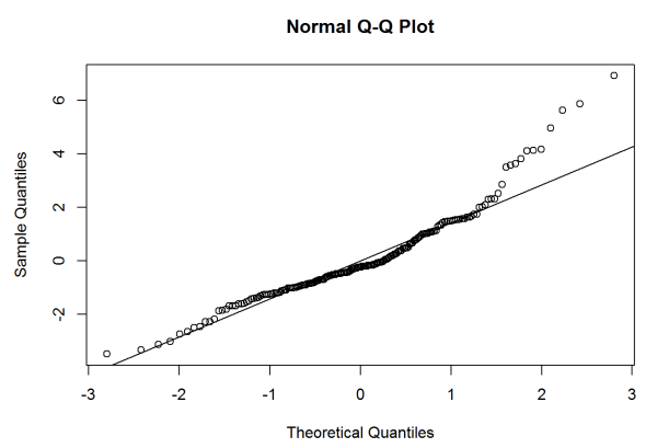
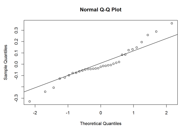
The other thing to note is that there is an additional assumption of normality not only on the model residuals, but also on the random effects. This can all be checked with a QQ-plot.
Let’s first check out the linearity and homogeneous variance assumptions
using a residuals vs. fitted plot. This can easily be recreated using
the plot() function on our model.
plot(model.4)
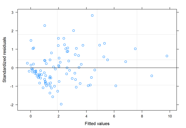
A lot of observations seem to cluster in the lower left area of the plot, so there may be some issue with the homogenous variance assumption. There is no real pattern in the plot so it looks like the linearity assumption is met.
It may be more helpful to check residual variance over time, since we took into account increasing variance over seasons. We can create a boxplot to look at this like so:
pacer.stats %>%
  mutate(res=residuals(model.4, type = "pearson"), fit=fitted(model.4)) %>%
  ggplot(aes(x=factor(Season.Number), y=res)) +
  geom_jitter(width = .2) +
  geom_boxplot(alpha=.5)
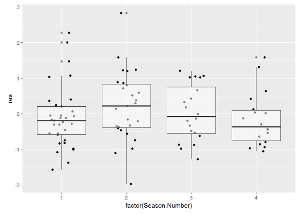
The variance between seasons doesn’t seem so bad here.
We can get QQ-plots of both the residuals and random effects by using
the qqnorm() function. We can call the random effects again using the
ranef() function.
qqnorm(model.4$residuals)
qqline(model.4$residuals)
qqnorm(ranef(model.4)$`(Intercept)`)
qqline(ranef(model.4)$`(Intercept)`)
qqnorm(ranef(model.4)$Season.Number)
qqline(ranef(model.4)$Season.Number)
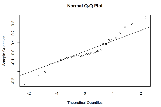
It looks like there might be some normality assumptions, especially with
the random slope for Season.Number. Adding some transformations might
help, but I’ll save that for a future post.
Making Predictions
Mixed-effects models can make predictions on new data, but they’ll only use the fixed effects if that person was not included in the model building process. The model does take the random effects into account if we wanted to add in observations from players in the study.
Let’s look at the four Pacer rookies from this season: Ben Moore, Edmond Sumner, Ike Anigbogu, and T.J. Leaf. What if wanted to predict their win shares over the next three seasons?
Well, let’s first create a dataframe that replicates these players three
additional times. Each replications add one onto the season.number
variable for each consecutive row.
#first create a dataframe where only this year's rookies are included
rookies.2018<-
  pacer.stats %>%
  filter(Rookie.Season==2018) %>%
  select(Player, Rookie.Season, Season.Number, Round, Rookie.Age, WS)

#edit the dataframe so that it includes each player four times
rookies.2018<-
  #repeating each row four times
  rookies.2018[rep(row.names(rookies.2018), 4),] %>%
  #ordering players by name
  arrange(Player) %>%
  #adding sequence of values 0 to 3 to the season number
  mutate(Season.Number=Season.Number+(seq(1:4)-1))
Now, we can make predictions as to how the rookies will perform in the future. T.J. Leaf sees the largest amount of predicted win shares, but his rate of increase is pretty low compared to other players.
predict(model.4, newdata = rookies.2018)

##     Ben Moore     Ben Moore     Ben Moore     Ben Moore Edmond Sumner
##     0.3051530     0.9715436     1.6379341     2.3043246     0.1164006
## Edmond Sumner Edmond Sumner Edmond Sumner  Ike Anigbogu  Ike Anigbogu
##     0.8394452     1.5624898     2.2855345     0.1469455     0.8908371
##  Ike Anigbogu  Ike Anigbogu     T.J. Leaf     T.J. Leaf     T.J. Leaf
##     1.6347287     2.3786203     1.3583205     1.9487227     2.5391250
##     T.J. Leaf
##     3.1295272
## attr(,"label")
## [1] "Predicted values"
Conclusion
Mixed-effects models are great for grouped and time series analysis. Assumptions of independence and homogenous variance can be very limiting, but mixed-effects models allow us to relax these assumptions. Go forth with your longitudinal study; the world is your oyster!
