Comparing Means With the T-Test
In this tutorial, we’re going to go over using t-tests. The t-test compares the averages of two groups and identifies whether they are different beyond random chance. Although basic, the t-test can be useful in a lot of projects.
The Data
The data we’ll be using in this tutorial are the individual game scores for the 2010-11 season for Derrick Rose and LeBron James. This was Rose’s MVP season, although many viewed James as more deserving of the award. We’ll use basketball-reference’s game scores to see if there was a significant difference between Rose and James’ performance during the season (at least by this metric).

First we’re going to bring up the libraries we’ll need. We’ll need a couple of packages from the tidyverse series of packages, so we’ll just load them all up by loading tidyverse.
library(tidyverse)
Next, let’s gather the data. I put Rose’s info in a tibble called rose and James’ in a tibble called james. The PLAYER column is their last name and the GMSC column is the game scores they had for the 2010-11 season. I also combined these two tibbles into one called combo that will be helpful for some data manipulation/plotting purposes.
rose <- tibble(PLAYER= "Rose",
               GMSC=c(14, 26.4, 14.7, 22.2, 9.7, 8, 23.2, 19.7, 27.6,
                      19, 14.9, 21.5, 20.7, 24.5, 6, 12.6, 26.3, 7.9,
                      21.4, 19.3, 20.7, 13.8, 7.3, 26.4, 26.2, 15.6,
                      16.1, 14.9, 18.1, 16.7, 21.4, 17.2, 9.1, 22,
                      24.4, 25.9, 9.9, 23.2, 26.8, 22.1, 20.2, 16.6,
                      18.9, 18.5, 17.9, 16.5, 30.9, 5, 22, 21, 16.9,
                      13.6, 36.4, 23.9, 13.3, 9.9, 19.4, 4.2, 13.8,
                      16.7, 19, 20.8, 23.7, 16.2, 17, 13.5, 24, 16.1,
                      28, 14.4, 32.5, 16.6, 22.8, 23.1, 32.6, 12.9,
                      27.7, 6.7, 31.6, 15.9, 8.6))

james <- tibble(PLAYER= "James",
                GMSC=c(16, 9.6, 10, 15.6, 23.7, 20.6,
                       19.4, 22.8, 29, 17.6, 20.6, 20.6, 21.7, 15.5,
                       17, 18, 11.7, 19.8, 12, 33.7, 19.7, 12.5,
                       28.6, 21.7, 19, 11.1, 14.5, 27, 24.4, 11.2,
                       26.8, 33.3, 12.9, 17.6, 23.1, 28.8, 24, 20.1,
                       35.1, 17.4, 20.5, 30.1, 15, 34, 25.6, 22.8,
                       46.7, 17.2, 5.3, 39.3, 16.9, 14.5, 20.3, 17.7,
                       17.9, 25.5, 27, 19.7, 26.2, 20.2, 24, 26.5,
                       17.8, 23.8, 16.5, 12.7, 32.2, 20.5, 14.9,
                       28.2, 28.6, 21.9,34.6, 26.1, 26.6, 22, 24.7, 23.2,
                       26.4))

combo <- rose %>%
  bind_rows(james)
One Sample T-Test
Let’s first look at Rose by himself. Let’s say that out of of all basketball players, the average game score is 12 (just a complete guess). I want to know whether Rose’s mean game score is significantly better than the population mean, and not just a result of random variation.
To answer this question, we can perform a one-sample t-test. Using R we call the t.test function, like so:
t.test(rose$GMSC, mu = 12, alternative = "greater")
##
##  One Sample t-test
##
## data:  rose$GMSC
## t = 8.8151, df = 80, p-value = 1.014e-13
## alternative hypothesis: true mean is greater than 12
## 95 percent confidence interval:
##  17.4552     Inf
## sample estimates:
## mean of x
##  18.72469
We first input Rose’s game scores, followed by mu (the population mean). We also are only interested if Rose’s mean score is greater than the population mean. Because of this, we can specify alternative = "greater. This is known as a one-tailed t-test; we’re only interested if the difference is significantly greater or less than 0, not whether there is any difference at all.
Using the typical hypothesis testing lingo (I promise not to use it a lot), the null hypothesis is Rose's mean game score is not greater than the population mean. The alternative hypothesis is Rose's mean game score is greater than the population mean. We set an alpha or significance value (usually .05) which we’ll compare the p-value to. If the p-value is below the significance level, we reject the null; if not, we fail to reject it.
The p-value stands for probability value and represents the probability we’d see this result or a more extreme one given that our null hypothesis is true. For a t-test, it is based off of the t-value (crazy, I know!). Now, what exactly is the t-value? I thought we were comparing averages! Well, different studies are going to have results that differ based on the event being studied. We might say that a difference of 15 between two players’ points per game average is a pretty large difference. We wouldn’t say that a difference of 15 in two stadiums’ average attendance numbers is that different, though! The t-value standardizes this difference and compares it to a set t-distribution to get the p-value. Larger absolute values of t indicate larger differences.
Although the p-value is the go to for most people to determine significant effect, never use it as a sole measure. The p-value is simply the probability we’d see this result or a more extreme one given that our null hypothesis is true. It’s not really a measure of effect size. Make sure to include things like confidence intervals, which shows a possible range as to where the true value lies, as a way to back up your claims, not just the p-value.
Now, looking at the results show that Rose’s mean game score is signicantly higher than the population mean. The 95% confidence interval shows a likely range for the true population mean game score of greater than 17.45. The p-value is below .05, showing that the difference is significant at the traditional .05 significance level.
Before we celebrate too much, there are some diagnostics we have to run. Specifically, we have to test for normality in the distribution of Rose’s game scores. We can do this graphically or with a more general hypothesis test: the Shapiro-Wilk test.
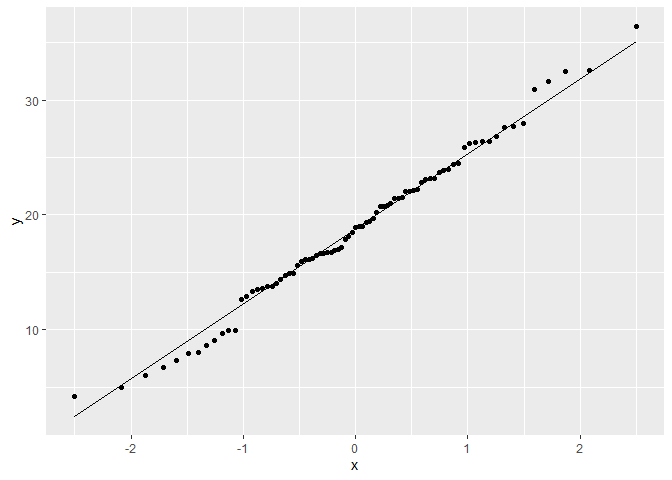
First we’ll show the graphical way. This is a quantile quantile (QQ) plot, comparing sample and theoretical quantiles. Ideally, we want all the points to line up diagonally on the quantile quantile line.
rose %>%
  ggplot(aes(sample = GMSC)) +
  geom_qq_line() +
  geom_qq()

The points seem to follow the line for the most part, indicating that the data is essentially normal. We can also use the Shapiro-Wilk test like so:
shapiro.test(rose$GMSC)
##
##  Shapiro-Wilk normality test
##
## data:  rose$GMSC
## W = 0.99037, p-value = 0.812
The null hypothesis for a Shapiro-Wilk test is that the data is approximately normal. Because the p-value is not below .05 we fail to reject the null. Our t-test is valid!
Two Sample T-Test

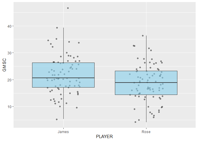
Now we’ll go back to our example mentioned at the beginning: comparing James and Rose’s game scores. Let’s first look at the distribution of game scores in a box plot.
combo %>%
  ggplot(aes(x = PLAYER, y = GMSC)) +
  geom_jitter(alpha = .4, width = .2) +
  geom_boxplot(fill = "skyblue", alpha = .6, outlier.colour = NA)

Based on the graph, it looks like James’ distribution of game scores is slightly higher than Rose’s.
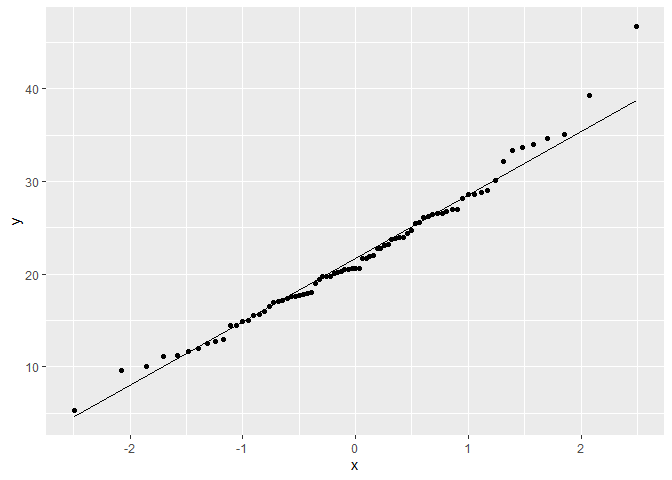
Before we run any tests on the data, let’s run diagnostics on James’ data.
james %>%
  ggplot(aes(sample = GMSC)) +
  geom_qq_line() +
  geom_qq()

shapiro.test(james$GMSC)
##
##  Shapiro-Wilk normality test
##
## data:  james$GMSC
## W = 0.97822, p-value = 0.1954
Based on the QQ plot and the Shapiro-Wilk test, it appears as though James’ game score data is approximately normal.
For two sample t-tests, we have an extra assumption that must be met. We also have to check for equal variance between the samples. We can do this with the var.test function:
var.test(rose$GMSC, james$GMSC)
##
##  F test to compare two variances
##
## data:  rose$GMSC and james$GMSC
## F = 0.88567, num df = 80, denom df = 78, p-value = 0.5901
## alternative hypothesis: true ratio of variances is not equal to 1
## 95 percent confidence interval:
##  0.5676193 1.3801857
## sample estimates:
## ratio of variances
##          0.8856696
This runs an F-test to compare the variances. The null hypothises is that the variances between the two inputs are approximately equal. The p-value is above .05 and the 95% confidence interval includes 1, so we can assume that the variances are equal. Since both samples are normal and the variances are equal, we can run a two-sample student’s t-test:
t.test(rose$GMSC, james$GMSC, var.equal = T)
##
##  Two Sample t-test
##
## data:  rose$GMSC and james$GMSC
## t = -2.6911, df = 158, p-value = 0.007888
## alternative hypothesis: true difference in means is not equal to 0
## 95 percent confidence interval:
##  -5.2248125 -0.8017541
## sample estimates:
## mean of x mean of y
##  18.72469  21.73797
Although we used the same t.test command, the inputs are slighty different. We specify var.equal = T because variances are equal. We also didn’t specify an alternative, making this a two-sided test. We are interested in any difference, not whether one mean is significantly greater or lesser.
The 95% confidence interval in the difference between Rose and James’ means is -5.22 and -.80; because it does not include 0, and because the p-value is below .05, we can say there is a significant difference between Rose and James’ game scores. Rose’s game scores are significantly lower.
Although game scores are just one measure, it appears as though LeBron was better in this category than Rose. Maybe there’s some truth to the rumor that people were just fed up with LeBron winning all of the awards, so they voted for the next best thing.
What if Assumptions aren’t met?
There are alternative t-tests that can be used if the variance and normality assumptions aren’t met. If the two samples have unequal variances, a Welch t-test can be used. We can simply set the var.equal command to false:
t.test(rose$GMSC, james$GMSC, var.equal = F)
##
##  Welch Two Sample t-test
##
## data:  rose$GMSC and james$GMSC
## t = -2.6891, df = 156.85, p-value = 0.00794
## alternative hypothesis: true difference in means is not equal to 0
## 95 percent confidence interval:
##  -5.2266254 -0.7999412
## sample estimates:
## mean of x mean of y
##  18.72469  21.73797
If the samples aren’t normally distributed, we should use a Mann-Whitney-Wilcoxon test. This is a non-parametric method in which we don’t have to assume a normal distribution. Instead, we compare the ranks of the input values.
wilcox.test(rose$GMSC, james$GMSC)
##
##  Wilcoxon rank sum test with continuity correction
##
## data:  rose$GMSC and james$GMSC
## W = 2490, p-value = 0.01553
## alternative hypothesis: true location shift is not equal to 0
The results are both similar to the student’s t-test we ended up using, but the output is slightly different. It’s good practice to use the appropriate test when necessary, so make sure to always check your diagnostics!
